In my previous post on speculative decoding, I kept hammering on one point: LLM inference is memory-bound. The GPU sits idle 98% of the time, waiting for weights to load from memory. Speculative decoding helps by verifying multiple tokens per memory load.
But that got me thinking - what about making each individual operation faster? If we’re memory-bound, surely we can do better than PyTorch’s default kernels?
Turns out, we can. A lot better. I spent a few weeks writing custom kernels in OpenAI Triton and the results surprised me. PyTorch’s RMSNorm achieves 11% of peak memory bandwidth. My Triton version hits 88%. That’s an 8x speedup on a single operation.
This post walks through what I learned. The code is at github.com/bassrehab/triton-kernels.
Why Bother with Custom Kernels?
Quick recap from the speculative decoding post: a 7B parameter model in FP16 is 14GB. On an A100 with 2TB/s bandwidth, loading those weights takes ~7ms. The actual math? Maybe 0.1ms.
So why is PyTorch leaving 89% of bandwidth on the table for something as simple as RMSNorm?
Three reasons:
-
Kernel launch overhead. PyTorch dispatches multiple small CUDA kernels. Each launch has ~5-10μs overhead. For small operations, this dominates.
-
Intermediate tensors. PyTorch materializes intermediate results to GPU memory, then reads them back. More memory traffic = slower.
-
Generic implementations. PyTorch kernels handle every edge case. Custom kernels can be optimized for specific shapes and dtypes.
Triton lets you write fused kernels that avoid all three problems. And unlike raw CUDA, you don’t need to think about warps, shared memory tiling, or register allocation. Triton handles that.
The Kernels I Built
I focused on four operations common in modern LLMs:
| Kernel | What it does | Speedup |
|---|---|---|
| RMSNorm | Root mean square normalization | 8.1x |
| RMSNorm + Residual (fused) | Normalize after residual add | 6.0x |
| SwiGLU (fused) | Gated activation (LLaMA-style) | 1.6x |
| INT8 GEMM | Quantized matrix multiply | ~1.0x (2x memory savings) |
Let me walk through the most interesting one - RMSNorm - to show how Triton optimization works.
Deep Dive: RMSNorm
RMSNorm is dead simple mathematically:
\[y = \frac{x}{\sqrt{\frac{1}{n}\sum x^2 + \epsilon}} \cdot \gamma\]That’s it. Compute the root mean square, divide, scale by a learned weight. Every transformer uses this (or LayerNorm, which is similar).
The PyTorch Version
Here’s how you’d write it in PyTorch:
def rmsnorm_pytorch(x, weight, eps=1e-6):
    variance = x.pow(2).mean(dim=-1, keepdim=True)
    x_normed = x * torch.rsqrt(variance + eps)
    return x_normed * weight
Three lines. Clean. But let’s count the memory operations:
x.pow(2)- read x, write x².mean()- read x², write variancetorch.rsqrt()- read variance, write rsqrtx * rsqrt- read x again, read rsqrt, write normalized* weight- read normalized, read weight, write output
That’s reading x twice, plus a bunch of intermediate tensors. For a tensor of shape (batch, seq, hidden), we’re moving way more data than necessary.
The Triton Version
Here’s the key insight: we can compute everything in one pass. Read x once, accumulate the sum of squares in registers, compute the normalization factor, write the output. One read, one write.
@triton.jit
def rmsnorm_kernel(
    X, Y, W,
    stride, n_cols,
    eps,
    BLOCK_SIZE: tl.constexpr,
):
    # Each program handles one row
    row = tl.program_id(0)

    # Pointers for this row
    X_row = X + row * stride
    Y_row = Y + row * stride

    # Accumulate sum of squares in registers (FP32 for precision)
    sum_sq = tl.zeros([BLOCK_SIZE], dtype=tl.float32)

    for off in range(0, n_cols, BLOCK_SIZE):
        cols = off + tl.arange(0, BLOCK_SIZE)
        mask = cols < n_cols
        x = tl.load(X_row + cols, mask=mask, other=0.0).to(tl.float32)
        sum_sq += x * x

    # Compute normalization factor
    mean_sq = tl.sum(sum_sq) / n_cols
    rstd = 1.0 / tl.sqrt(mean_sq + eps)

    # Second pass: normalize and write output
    for off in range(0, n_cols, BLOCK_SIZE):
        cols = off + tl.arange(0, BLOCK_SIZE)
        mask = cols < n_cols
        x = tl.load(X_row + cols, mask=mask, other=0.0).to(tl.float32)
        w = tl.load(W + cols, mask=mask, other=1.0).to(tl.float32)
        y = x * rstd * w
        tl.store(Y_row + cols, y.to(tl.float16), mask=mask)
A few things to notice:
-
Two passes, not five. We read x twice (once for variance, once for normalization), but no intermediate tensors hit memory.
-
FP32 accumulation. The sum of squares uses float32 to avoid precision loss. The output is still float16.
-
Block-based processing. Triton processes BLOCK_SIZE elements at a time. The compiler figures out how to map this to GPU threads.
The Results
On an A100 with LLaMA-7B dimensions (hidden_dim=4096, seq_len=2048):
| Implementation | Latency | Bandwidth | % of Peak |
|---|---|---|---|
| PyTorch | 0.30 ms | 168 GB/s | 11% |
| Triton | 0.04 ms | 1365 GB/s | 88% |
8.1x faster. And we’re hitting 88% of the A100’s theoretical peak bandwidth (1555 GB/s). That’s about as good as it gets for a memory-bound operation.
Fusion: The Real Win
RMSNorm is fast, but the bigger win comes from fusion. In a transformer block, you typically see:
# Residual connection + normalization
hidden = hidden + residual
hidden = rmsnorm(hidden)
PyTorch runs these as separate kernels:
- Read hidden, read residual, write sum
- Read sum, compute norm, write output
With Triton, we fuse them into one kernel:
- Read hidden, read residual, compute norm, write output
One less round-trip to memory. The fused kernel runs at 6.0x the speed of PyTorch’s separate operations.
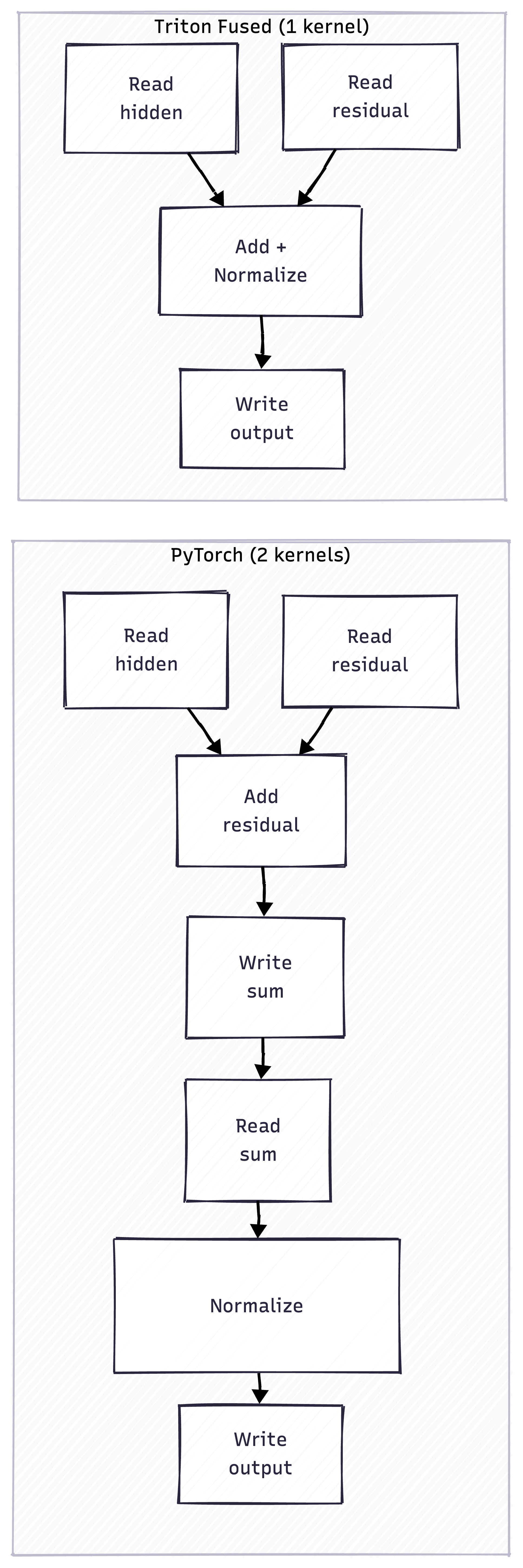
The red boxes (W1, H2) in PyTorch are unnecessary memory operations that fusion eliminates.
SwiGLU: Another Fusion Opportunity
Modern LLMs like LLaMA use SwiGLU instead of ReLU:
\[\text{SwiGLU}(x, W, V) = (\text{SiLU}(xW)) \odot (xV)\]In PyTorch:
gate = F.silu(x @ W)  # Write intermediate
up = x @ V            # Write intermediate
output = gate * up    # Read both, write output
In Triton, we fuse the final multiply:
# After the matmuls...
output = silu(gate) * up  # One kernel, no intermediates
The speedup here is more modest (1.6x) because the matmuls dominate. But it’s still free performance.
INT8 Quantization: Memory Savings Over Speed
I also implemented INT8 matrix multiplication. The speedup is… basically nothing. Maybe 1.04x. But that’s not the point.
The point is memory savings. INT8 weights are half the size of FP16. For a 70B model, that’s the difference between fitting in one GPU or needing two.
The catch is that you need to dequantize on-the-fly:
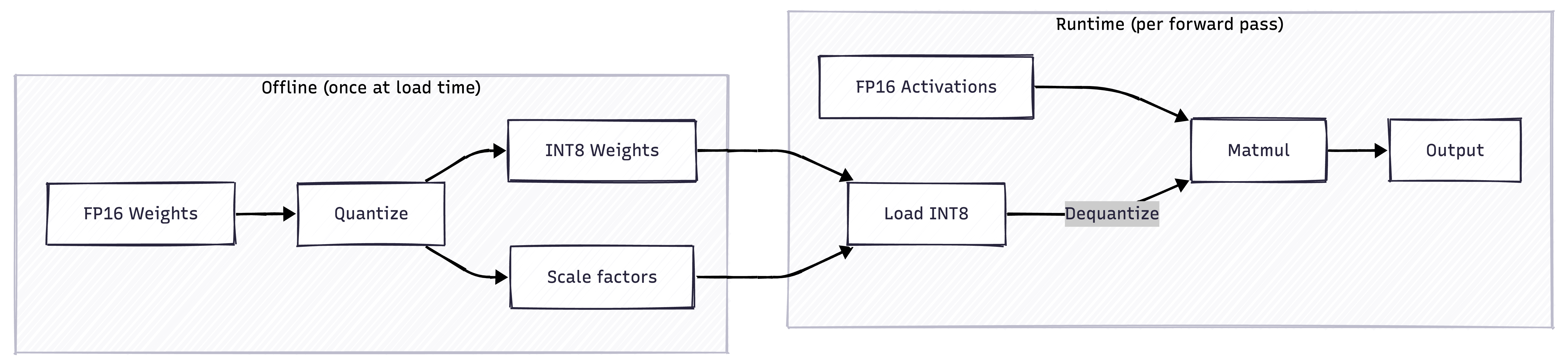
The dequantization adds overhead, which is why the speedup is minimal. But for memory-constrained deployments, it’s worth it.
Why not use INT8 activations too? (click to expand)
Full INT8 inference (W8A8) uses the GPU's tensor cores for int8 matmul, which should be faster. But there's a catch: you need to quantize the activations at runtime. For each matmul, you'd need to: 1. Find the max absolute value of the activations 2. Compute a scale factor 3. Quantize to int8 4. Do the int8 matmul 5. Dequantize the output Steps 1-3 add overhead that often outweighs the tensor core speedup, especially for small batch sizes. W8A16 (int8 weights, fp16 activations) avoids this by only quantizing weights once at load time. For more details, see my [INT8 investigation notes](https://github.com/bassrehab/triton-kernels/blob/main/docs/INT8_GEMM_INVESTIGATION.md).Lessons Learned
1. Measure bandwidth, not FLOPS
The number that matters for memory-bound operations is GB/s, not TFLOPS. My RMSNorm kernel does barely any floating-point math - it’s almost entirely memory traffic. Measuring FLOPS would be misleading.
2. PyTorch overhead is real
For small operations, kernel launch overhead dominates. Fusing operations isn’t just about reducing memory traffic - it’s also about launching fewer kernels.
3. Triton is surprisingly accessible
I expected writing GPU kernels to be painful. Triton abstracts away most of the hard parts - thread indexing, shared memory, register allocation. You think in terms of blocks and masks, not warps and occupancy.
That said, there’s still a learning curve. The Triton tutorials are good. Horace He’s GPU optimization guide is essential background.
4. Don’t roll your own for production
These are educational implementations. For real deployments, use FlashAttention, vLLM, or TensorRT-LLM. They’ve solved problems I haven’t touched - multi-query attention, paged KV-cache, speculative decoding integration, etc.
But if you want to understand why those libraries are fast, writing your own kernels is a great exercise.
What’s Next
I want to tackle fused attention at some point. FlashAttention is the gold standard, but it’s complex - online softmax, block-sparse patterns, backward pass. Not a weekend project.
The more immediate gap in my repo is end-to-end integration. Right now these are standalone kernels. Wiring them into an actual model (say, LLaMA inference) would be a good next step.
Code
Everything is on GitHub: github.com/bassrehab/triton-kernels
The main files:
triton_kernels/rmsnorm.py- RMSNorm + fused residualtriton_kernels/swiglu.py- SwiGLU activationtriton_kernels/quantized_matmul.py- INT8 GEMMbenchmarks/- Benchmark suite with roofline analysis
There’s also a detailed ROOFLINE_ANALYSIS.md that explains the performance characteristics of each kernel.
Takeaways
If you’re doing LLM inference optimization, the mental model shift is important: stop thinking about FLOPS and start thinking about memory bandwidth. Most operations are memory-bound, and the win comes from:
- Fusion - fewer round-trips to memory
- Quantization - less data to move
- Efficient access patterns - maximize bandwidth utilization
PyTorch is leaving a lot of performance on the table for common operations. Custom Triton kernels can close that gap. For RMSNorm, the gap was 8x.
But unless you have specific needs, use the battle-tested libraries. The wins from custom kernels often don’t justify the maintenance burden. Write your own to learn, but deploy with FlashAttention and vLLM.
This is Part 2 of my LLM inference series. Part 1 covered speculative decoding - a different angle on the same memory-bound problem. Questions or feedback? Open an issue on the repo or reach out.