The Manifold Dial: Visualizing Why DeepSeek's mHC Stabilizes Deep Networks

Nine Years of “Good Enough”

Residual connections haven’t changed since 2016. He et al. introduced them in ResNet, the formula stuck (output = layer(x) + x), and we’ve been using the same thing ever since. Attention mechanisms evolved. Normalization techniques multiplied. FFN architectures got reworked a dozen times. But skip connections? Untouched.

It’s not that nobody tried. There’s been work on dense connections, highway networks, various gating mechanisms. Most added complexity without clear wins. The simple additive skip connection kept winning.

Then Hyper-Connections came along and showed genuine improvements by expanding the residual stream - multiple parallel paths instead of one, with learned mixing between them. Promising results. But also a problem that becomes obvious only at scale: the networks become unstable during training. Loss spikes. Gradient explosions. The deeper you go, the worse it gets.

DeepSeek’s mHC paper explains why this happens and how to fix it. The fix involves projecting matrices onto something called the Birkhoff polytope using an algorithm from 1967. I built an interactive tool to visualize what’s actually going on, because the equations alone don’t convey how dramatic the difference is.

What Hyper-Connections Actually Do

Standard residual: you compute a layer’s output and add back the input. One stream in, one stream out.

Hyper-Connections expand this to $n$ parallel streams (typically 4). Instead of simple addition, you get learned mixing matrices that control how information flows between streams:

Three matrices per layer: one to mix the residual streams ($H^{res}$), one to aggregate streams into the layer input ($H^{pre}$), one to distribute the layer output back to streams ($H^{post}$).

The paper’s ablation study shows $H^{res}$ matters most. That’s the mixing within the residual stream itself - how information from different streams combines as it flows through the network.

More expressivity should mean better performance, and it does. HC improves over standard residuals in their experiments. The catch is what happens when you stack 60+ layers.

The Composite Mapping Problem

Each layer multiplies by its $H^{res}$ matrix. Through $L$ layers, the effective transformation is:

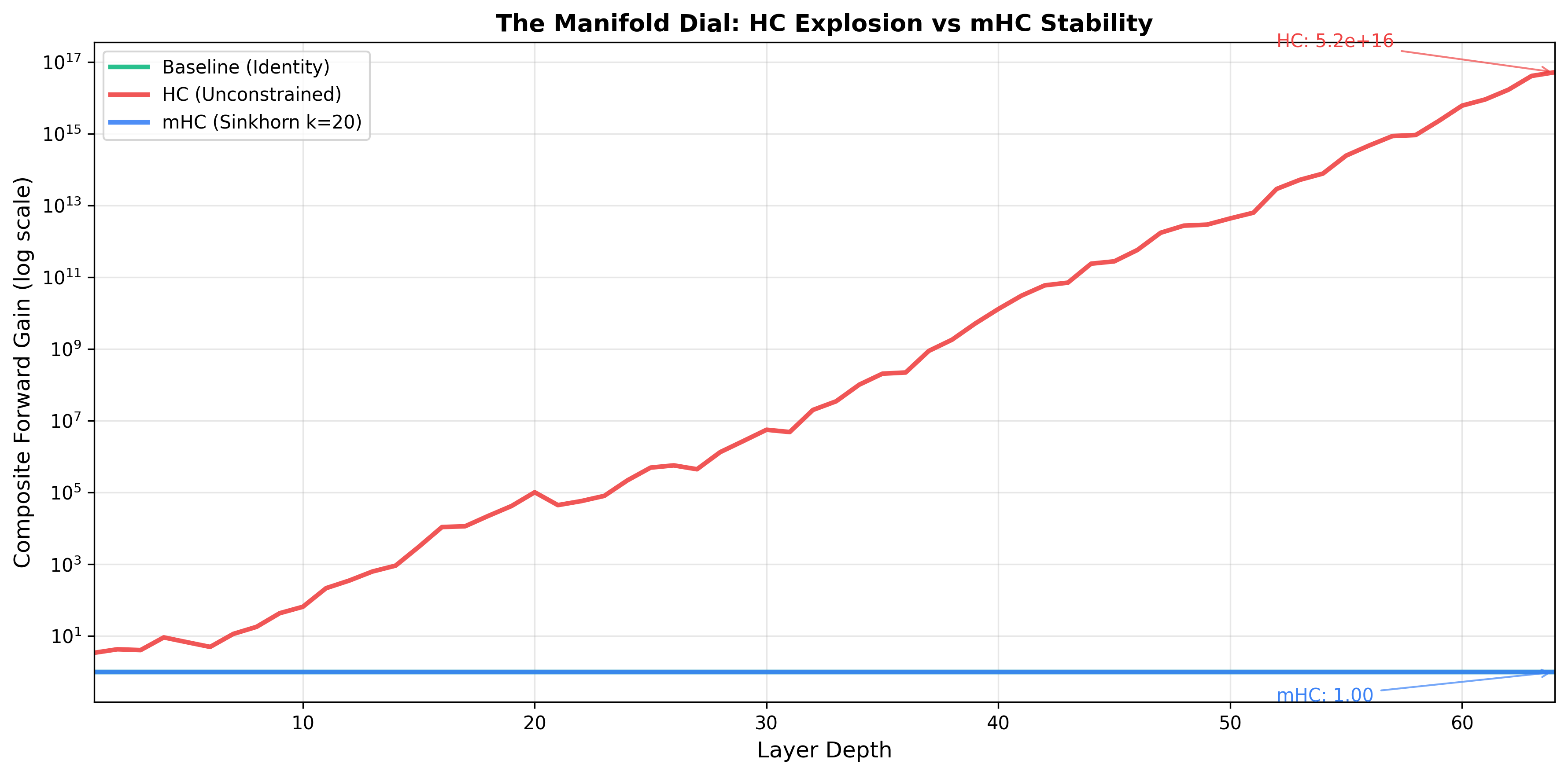
This product determines how signals from early layers reach later ones. With unconstrained learned matrices, small amplifications compound. A matrix with spectral norm 1.05 seems harmless. Sixty of them multiplied together? That’s $1.05^{60} \approx 18$. And real HC matrices aren’t limited to 1.05.

The paper measured this directly. Figure 3 shows the “Amax Gain Magnitude” - essentially the worst-case amplification through the composite mapping. For HC at depth 64, gains can reach 10³ to 10⁵ depending on initialization. In our toy simulation with random matrices, it’s even more extreme - up to 10¹⁶. The composite mapping amplifies signals catastrophically.

That’s why training becomes unstable. Gradients flow backward through the same composite mapping. A 3000x amplification in the forward pass means 3000x amplification in the backward pass. Gradient clipping helps, but you’re fighting the architecture itself.

The Fix: Doubly Stochastic Matrices

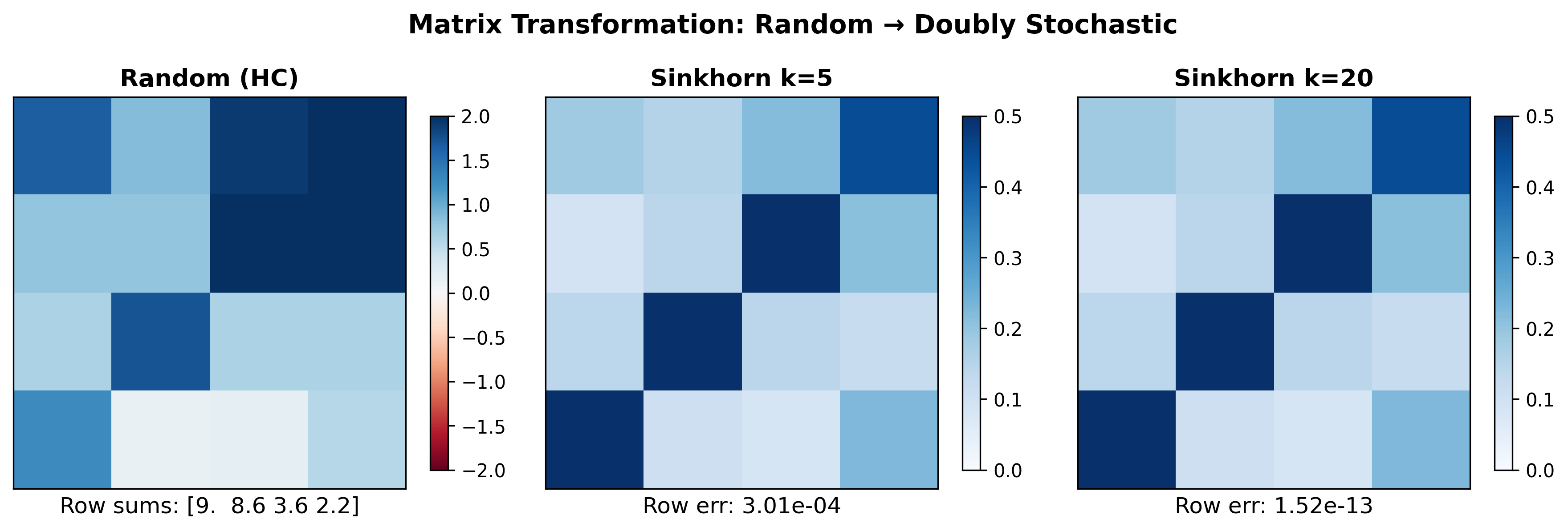
mHC constrains $H^{res}$ to be doubly stochastic - all entries non-negative, all rows sum to 1, all columns sum to 1.

Why this specific constraint? Three properties matter:

Spectral norm is bounded by 1. A doubly stochastic matrix cannot amplify signals. Each row summing to 1 means the weighted combination of inputs never exceeds the maximum input. No amplification, no explosion.

Closure under multiplication. Multiply two doubly stochastic matrices and you get another doubly stochastic matrix. This is the key insight. It doesn’t matter how many layers you stack - the composite mapping stays doubly stochastic, stays bounded.

Geometric interpretation. The set of doubly stochastic matrices forms the Birkhoff polytope, which is the convex hull of permutation matrices. Every doubly stochastic matrix can be written as a weighted average of permutations. Permutations just shuffle; they don’t amplify. Weighted averages of shuffles don’t amplify either.

The result: composite gains stay near 1 regardless of depth. The paper shows mHC at depth 64 has composite gain around 1.6. Compare that to HC’s explosive growth.

Sinkhorn-Knopp: 1967 Meets 2025

To make a learned matrix doubly stochastic, mHC uses the Sinkhorn-Knopp algorithm. Published in 1967 for balancing matrices in numerical analysis, it turns out to be exactly what’s needed here.

The algorithm is simple: exponentiate entries to make them positive, then alternate between normalizing rows and normalizing columns. Repeat until convergence. The iteration provably converges to a doubly stochastic matrix.

def sinkhorn_knopp(matrix, iterations=20, eps=1e-8):
    # Exponentiate (subtract max for numerical stability)
    P = np.exp(matrix - matrix.max())

    for _ in range(iterations):
        P = P / (P.sum(axis=1, keepdims=True) + eps)  # Row normalize
        P = P / (P.sum(axis=0, keepdims=True) + eps)  # Column normalize

    return P

Twenty iterations gets you close enough. The paper uses this as the default and shows it’s sufficient for the constraint to stabilize training.

The Manifold Dial

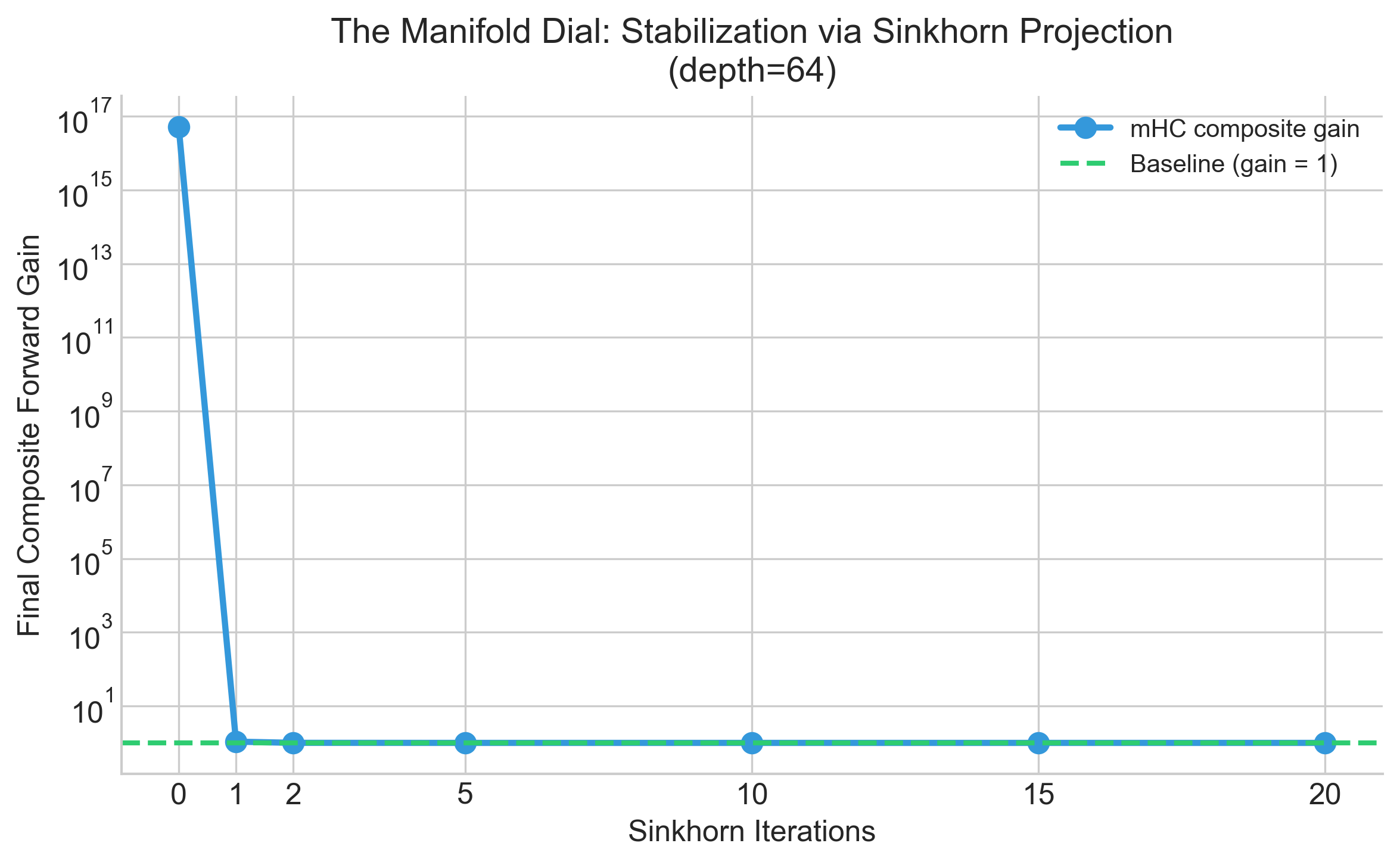
Here’s what I find most interesting: how quickly stability kicks in.

I swept the number of Sinkhorn iterations from 0 to 20 and measured the composite gain at depth 64. At zero iterations, you have an unconstrained matrix - basically HC. At twenty iterations, you have a nearly perfect doubly stochastic matrix - full mHC.

Interactive Demo

I built an interactive version so you can explore this yourself:

Open in new window ↗

Drag the Sinkhorn iterations slider. At 0, the mHC line explodes just like HC. As you increase iterations, watch it collapse down toward the stable baseline. Somewhere around 5-10 iterations, stability kicks in. By 20, it’s fully bounded.

The “manifold dial” is literally how much you’re projecting onto the doubly stochastic manifold. Zero projection means unconstrained chaos. Full projection means guaranteed stability.

This isn’t in the paper. I built it because the static figures don’t capture how smooth this transition is, or how little projection you actually need to get most of the stability benefit.

Comparison with the Paper

For reference, here’s a recreation of the paper’s Figure 3, showing both single-layer and composite gains:

Note that single-layer gains (left) aren’t catastrophic - individual HC matrices have gains in the 1-7 range. The problem is multiplication. Sixty matrices with average gain 3 gives $3^{60} \approx 10^{28}$. The composite mapping (right) reveals what single-layer analysis misses.

Practical Details

DeepSeek didn’t just prove this works mathematically - they scaled it to 27B parameter models and measured the system overhead.

Training stability improves dramatically. Their Figure 2 shows HC experiencing a loss spike around step 12k with gradient norm shooting up. mHC has no such spike. The gradient norm stays smooth throughout.

The overhead is manageable. The Sinkhorn iterations add computation, but they operate on small matrices ($n \times n$ where $n=4$ typically). With kernel fusion and careful memory management, the full mHC implementation adds 6.7% training time overhead. For the stability and performance gains, that’s a reasonable trade.

Benchmark results on the 27B model show mHC outperforming both baseline and HC across tasks. BBH improves from 43.8 (baseline) to 48.9 (HC) to 51.0 (mHC). Similar pattern across DROP, GSM8K, MMLU, and others.

What I Find Interesting

A few things stood out reading this paper:

The instability isn’t subtle. Three orders of magnitude in signal amplification isn’t a minor numerical issue you can tune away. It’s a fundamental architectural problem. HC was probably hitting this wall in ways that weren’t always diagnosed correctly.

The fix comes from constraints, not regularization. You could try to penalize large gains with loss terms, but that’s fighting the architecture. Constraining to doubly stochastic matrices makes explosion structurally impossible. The geometry of the constraint does the work.

The 1967 algorithm works. Machine learning keeps rediscovering techniques from optimization and numerical analysis. Sinkhorn-Knopp wasn’t designed for neural networks, but it slots in perfectly here. There’s probably more useful machinery sitting in old papers.

Macro-architecture gets less attention than it deserves. We spend enormous effort on attention variants and FFN structures, but how layers connect to each other - the topology of the network - might have similar headroom for improvement.

Code

I implemented both the visualization and a PyTorch module you can actually use:

from mhc import mHCResidual

# Drop-in residual connection replacement
residual = mHCResidual(dim=512, n_streams=4, sinkhorn_iters=20)

# In your forward pass
hidden = residual(hidden_states, layer_output)

The repository includes the interactive demo source, Python implementation with tests, and a Colab notebook if you want to experiment without local setup.

Links

• Interactive Demo - the manifold dial visualization
• GitHub Repository - full source, PyTorch module, tests
• Colab Notebook - run it yourself
• mHC Paper - the original DeepSeek paper

References

Xie, Z., Wei, Y., Cao, H., et al. (2025). mHC: Manifold-Constrained Hyper-Connections. arXiv preprint arXiv:2512.24880.

He, K., Zhang, X., Ren, S., & Sun, J. (2016). Deep Residual Learning for Image Recognition. CVPR.

Sinkhorn, R., & Knopp, P. (1967). Concerning nonnegative matrices and doubly stochastic matrices. Pacific Journal of Mathematics, 21(2), 343-348.