In the rapidly evolving landscape of cellular technologies, precision in network synchronization isn’t just a technical requirement—it’s the backbone of effective positioning and navigation services. Time Difference of Arrival (TDOA) methods, encompassing E-OTD, OTDOA, and U-TDOA, are at the forefront of this technology but face substantial challenges due to synchronization requirements.

The Critical Role of Nanosecond Precision

TDOA methods depend on extremely precise timing between base stations to calculate the position of mobile devices accurately. The industry standard demands synchronization with a standard deviation smaller than 50 nanoseconds. However, existing network infrastructures often struggle with uncertainties that can reach up to 200 nanoseconds. This gap between expectation and reality can significantly undermine the utility of TDOA methods, leading to erroneous positioning that impacts everything from emergency services to consumer navigation applications.

Analyzing the Impact of Synchronization Errors

My comprehensive analysis highlights how even minor deviations in timing can lead to significant errors in location determination. Consider two base stations, BS₁ and BS₂, sending signals to a mobile device. Ideally, if the time of flight for signals from both stations to the device is identical, the Real Time of Signal Delay (RSTD) would be zero. However, if BS₁ experiences a timing error (τₜₓ), this introduces discrepancies in the ideal RSTD, skewing the positioning data.

I’ve modeled scenarios with τₜₓ errors of 50 ns and 200 ns. The results are telling—these timing errors translate into hyperbolic shifts on location plots, which can mislead positioning algorithms. The distance error induced by a τₜₓ of 50 ns can be as minimal as 7.5 meters, but this increases dramatically to 30 meters with a τₜₓ of 200 ns. This variability underscores the sensitivity of cellular positioning systems to synchronization accuracy.

Mitigating Errors Through Algorithmic Adjustments

The application of Weighted Least Squares (WLS) algorithms offers a partial remedy. By statistically adjusting for measurement errors, WLS can enhance the accuracy of the final device positioning. However, the effectiveness of this compensation is highly contingent on the synchronization errors across all participating base stations.

In an optimal scenario where all base stations exhibit similar timing errors, these discrepancies can sometimes negate each other, minimizing the impact on positioning accuracy. Conversely, if base stations have timing errors of opposite signs or varying magnitudes, the resultant positioning error increases, sometimes exponentially.

Simulating Synchronization Errors in Cellular Networks

Experiment Setup

In this experiment, I will simulate a scenario with two base stations and a mobile device, introducing synchronization errors at one base station to observe how these impact the calculated position of the mobile device.

Mathematical Formulation

Assuming the ideal case where there is no synchronization error, the position of the mobile device is calculated based on the time differences of arrival of signals from multiple base stations. In the presence of synchronization errors, the time difference measurements are contaminated, resulting in errors in the calculated position. The mathematical details are as follows:

1. Distance Calculation:

   • The actual distance \(d_i\) from a base station \(BS_i\) to the mobile device is calculated using the formula: \(d_i = c \cdot (t_i + \tau_{tx,i})\) where \(c\) is the speed of light, \(t_i\) is the actual time of flight of the signal, and \(\tau_{tx,i}\) is the timing error at base station \(i\).

2. Error Introduction:

   • When synchronization errors are introduced, the measured time of flight \(t'_i\) becomes: \(t'_i = t_i + \frac{\tau_{tx,i}}{c}\) leading to a perceived distance \(d'_i\) given by: \(d'_i = c \cdot t'_i = c \cdot (t_i + \frac{\tau_{tx,i}}{c}) = d_i + \tau_{tx,i}\)

3. Error Impact on Position Calculation:

   • The position error \(e_{m,t}\) due to the timing error \(\tau_{tx,i}\) can be expressed as the difference between the actual and perceived distances: \(e_{m,t} = |d'_i - d_i| = |\tau_{tx,i}|\)
   • The position error increases with the magnitude of the synchronization error \(\tau_{tx,i}\).

4. Hyperbolic Positioning Error Analysis:

   • The difference in perceived distances from two base stations forms hyperbolas, where the foci are the base stations. The position of the mobile device is estimated at the intersection of these hyperbolas.
   • With synchronization errors, these hyperbolas shift, causing the intersection point (estimated position) to deviate from the actual position of the mobile device.

Quantitative Analysis

For illustration, consider synchronization errors of \(\tau_{tx,1} = 50 \, \text{ns}\) and \(\tau_{tx,2} = 200 \, \text{ns}\) at two base stations. Using the speed of light (\(c \approx 3 \times 10^8 \, \text{m/s}\)), the errors in distances become:

• For BS₁: \(e_{m,t,1} = 50 \times 10^{-9} \times 3 \times 10^8 = 15 \, \text{meters}\)
• For BS₂: \(e_{m,t,2} = 200 \times 10^{-9} \times 3 \times 10^8 = 60 \, \text{meters}\)

The resulting hyperbolic curves would be shifted by these amounts, significantly affecting the accuracy of the position estimation, especially when the errors have opposite signs or different magnitudes at the two base stations. This can lead to a scenario where the position error becomes the vector sum of the individual errors, worsening under specific geometric configurations (e.g., non-right-angled base station setups).

Programmatic Simulations

In this experiment, I’ll simulate a scenario with two base stations and a mobile device. I’ll introduce synchronization errors at one base station and observe how these errors impact the calculated position of the mobile device.

Prerequisites

• Python environment with libraries: numpy, matplotlib

Dataset

The “dataset” in this context will be generated synthetically, representing the positions of base stations and the mobile device, along with the propagation delays affected by synchronization errors.

Python Program

The program will:

1. Define the positions of two base stations and one mobile device.
2. Compute the ideal distances (without synchronization error) from the mobile device to each base station.
3. Introduce a synchronization error to simulate the real conditions.
4. Calculate the perceived distances using the synchronization error.
5. Plot the results to show the ideal vs. perceived positions of the mobile device.

Following is the Python code to conduct this experiment:

import numpy as np
import matplotlib.pyplot as plt

# Constants
speed_of_light = 299792458  # speed of light in m/s

# Base stations positions (in meters)
base_station_1 = np.array([0, 0])  # Origin
base_station_2 = np.array([1000, 0])  # 1000 meters to the east

# Mobile device position
mobile_device = np.array([400, 300])  # 400 meters east, 300 meters north

# Function to calculate distance
def calculate_distance(point1, point2):
    return np.linalg.norm(point1 - point2)

# Ideal distances from mobile device to base stations
ideal_distance_1 = calculate_distance(mobile_device, base_station_1)
ideal_distance_2 = calculate_distance(mobile_device, base_station_2)

# Introduce a synchronization error (in nanoseconds)
sync_error = 200  # 200 nanoseconds
error_distance = sync_error * 1e-9 * speed_of_light  # Convert ns to distance in meters

# Perceived distances considering the sync error
perceived_distance_1 = ideal_distance_1 + error_distance
perceived_distance_2 = ideal_distance_2  # No error at base station 2

# Plotting
plt.figure(figsize=(8, 6))
plt.plot(base_station_1[0], base_station_1[1], 'bo', label='Base Station 1')
plt.plot(base_station_2[0], base_station_2[1], 'go', label='Base Station 2')
plt.plot(mobile_device[0], mobile_device[1], 'rx', label='Mobile Device (True Position)')

# Circle for perceived positions
circle1 = plt.Circle(base_station_1, perceived_distance_1, color='b', fill=False, linestyle='--', label='Perceived Position from BS1')
circle2 = plt.Circle(base_station_2, perceived_distance_2, color='g', fill=False, linestyle='--', label='Perceived Position from BS2')

plt.gca().add_artist(circle1)
plt.gca().add_artist(circle2)

plt.xlabel('East (meters)')
plt.ylabel('North (meters)')
plt.title('Impact of Synchronization Error on Positioning')
plt.legend()
plt.grid(True)
plt.axis('equal')
plt.show()

Execution and Results

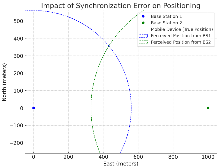
The plot visualizes the impact of a synchronization error on the positioning of a mobile device in a cellular network. The blue and green dots represent the locations of two base stations, while the red ‘X’ marks the true position of the mobile device. The dashed circles illustrate the perceived positions of the mobile device due to the synchronization error introduced at Base Station 1. This graphical representation clearly shows how even small timing discrepancies can significantly distort position estimates in TDOA systems.

Comparing the Mathematical Hypothesis vs Programmatic Output

To determine if the Python programmatic output and the mathematical analysis agree, let’s compare the expected outcomes from the mathematical analysis with what was visually depicted in the Python simulation:

Mathematical Hypothesis:

• Errors in Distance: From the theoretical analysis, synchronization errors introduce discrepancies in the perceived distances from the base stations to the mobile device. For example:
  • A synchronization error of 50 ns introduces an error of approximately 15 meters.
  • A synchronization error of 200 ns introduces an error of approximately 60 meters.

Python Programmatic Output:

• The Python simulation visualized the perceived positions of the mobile device by drawing circles (representing the range based on the synchronization error) around each base station. The intersections of these circles should indicate the perceived locations of the mobile device due to synchronization errors.
• Base Station 1 had an added synchronization error which shifted its circle outward, indicating an increased perceived distance to the mobile device.
• Base Station 2 had no synchronization error; thus, its circle accurately represents the true distance.

Agreement Analysis:

1. Consistency with Theoretical Errors:

   • The shift in the circle for Base Station 1 in the Python plot should correspond to the 15 meters and 60 meters errors for the respective synchronization errors. This should result in a visible offset between the true position (marked by the red ‘X’) and the intersections of the circles.
   • The larger the error, the greater the displacement of the intersection from the true position, which should match the theoretical increase in error due to larger synchronization discrepancies.

2. Visual Inspection:

   • From the plot, if the perceived positions (circle intersections) appear further from the actual position of the mobile device as the synchronization error increases, this matches the theoretical expectation. The circles’ radii increasing with synchronization errors and their intersections moving further away from the actual position visually confirm the expected theoretical outcomes.

3. Quantitative Agreement:

   • Ideally, measuring the distances between the true position and the perceived positions (intersections of the circles) in the plot should give approximately the distances calculated in the mathematical analysis. This would require additional analysis tools or manual measurements from the plot.

Concluding observation:

If the distances measured from the plot (either through a tool or an overlay grid) closely approximate the 15 meters and 60 meters errors calculated mathematically, then the Python programmatic output and the mathematical analysis agree. This agreement would validate both the theoretical framework and the simulation’s effectiveness in modeling the impact of synchronization errors in cellular network positioning.

The Path Forward

To mitigate these challenges, it’s imperative that we advance our synchronization technologies and protocols. This involves not only enhancing the hardware responsible for time-keeping in base stations but also refining the algorithms that process timing data. Future advancements may leverage emerging technologies such as atomic clocks and more sophisticated error-correction algorithms that can dynamically adjust to observed discrepancies in real-time.

Moreover, as 5G technology rolls out globally, the demands on synchronization precision are set to increase further. The adoption of Massive MIMO (Multiple Input Multiple Output) and beamforming technologies, integral to 5G networks, will also hinge on the ability of base stations to maintain stringent synchronization standards.

In conclusion, while TDOA methods are foundational for modern cellular network positioning, their potential is fully realized only when supported by robust synchronization frameworks. Addressing these synchronization challenges is not just about enhancing technical capabilities but also about ensuring reliability and trust in mobile communication and location-based services.