The explosion of big data has created an insatiable demand for analytical insights. However, traditional computational methods often struggle to keep up with the sheer volume and velocity of data in many real-world applications. This is where approximation techniques offer a lifeline — trading a small degree of accuracy for a significant boost in processing speed and efficiency.

Why Approximation?

In domains like real-time analytics, trend monitoring, and exploratory data analysis, the following often hold:

• Exactness is Overrated: A slightly less accurate answer available now often trumps a perfect result that arrives much later.
• Data is Messy: Real-world data is rarely pristine. Approximate techniques can often perform well even in the presence of noise and outliers.
• Resource Constraints: Hardware and computational constraints may make perfectly accurate computations either impractical or outright impossible.

Classes of Approximation Techniques

Let’s explore some key categories of approximate big data calculations:

1. Sampling

   • Idea: Instead of processing the entire dataset, work with a carefully selected subset.
   • Methods: Simple random sampling, Stratified sampling (ensure representation of subpopulations), Reservoir sampling (ideal for streaming data)
   • Example: Estimate the average customer purchase amount by analyzing a well-constructed sample of transactions rather than the entire sales history.

2. Sketching

   • Idea: Create compact ‘sketches’ or summaries of the data that capture key statistical properties.
   • Methods: Count-Min Sketch (frequency distributions), Bloom filters (probabilistic set membership), HyperLogLog (cardinality estimations)
   • Example: Track the number of unique visitors to a website using a HyperLogLog sketch, which efficiently compresses this information.

3. Synopsis Data Structures

   • Idea: Specialized data structures that maintain approximate summaries of data streams.
   • Methods: Histograms (approximate distributions), Wavelets (summarize time series or image data), Quantiles (approximate quantile calculation for ordering data)
   • Example: Monitor website traffic patterns over time using a histogram to approximate the distribution of page views.

Mathematical Considerations

Approximation techniques often come with provable accuracy guarantees. Key concepts include:

• Probability Bounds: Many sampling and sketching algorithms provide bounds on estimation error with a certain probability (e.g., “the true average lies within +/- 2% of our estimate with 95% confidence”).
• Convergence: Iterative algorithms often improve in accuracy with additional data or computation time, allowing you to tune their precision.

The Art of Approximation

Successful use of approximate calculations often lies in selecting the right technique and understanding its trade-offs, as different algorithms may offer varying levels of accuracy, space efficiency, and computational cost.

The embrace of approximation techniques marks a shift in big data analytics. By accepting a calculated level of imprecision, we gain the ability to analyze datasets of previously unmanageable size and complexity, unlocking insights that would otherwise remain computationally out of reach.

Big data calculations traditionally involve exact computations, where every data point is processed to yield precise results. This approach is comprehensive but can be highly resource-intensive and slow, especially as data volumes increase. In contrast, approximate calculations leverage statistical and probabilistic methods to deliver results that are close enough to the exact values but require significantly less computational power and time. Here’s a practical example comparing the two approaches:

Example: Calculating Average Customer Spend in Retail

Traditional Exact Calculation

Scenario: A large retail chain wants to calculate the average amount spent per customer transaction over a fiscal year. The dataset includes millions of transactions.

Method:

• Data Collection: Gather all transaction data for the year.
• Summation: Calculate the total amount spent by adding up every single transaction.
• Counting: Count the total number of transactions.
• Average Calculation: Divide the total amount spent by the number of transactions to get the exact average.

Approximate Calculation Using Sampling

Scenario: The same retail chain adopts an approximate method to calculate the average spend per customer transaction to reduce computation time and resource usage.

Method:

• Data Sampling: Randomly sample a subset of transactions from the dataset (e.g., 0.1% of total transactions).
• Summation: Calculate the total amount spent in the sample.
• Counting: Count the number of transactions in the sample.
• Average Calculation: Divide the total amount in the sample by the number of sampled transactions to estimate the average.

Comparison and Conclusion:

• Accuracy: The traditional method provides exact results, while the approximate method offers results with a margin of error that can typically be quantified (e.g., confidence intervals).
• Efficiency: Approximate calculations are much faster and less resource-intensive, making them suitable for quick decision-making and real-time analytics.
• Scalability: Approximate methods scale better with very large datasets and are particularly useful in environments where data is continuously generated at high volumes (e.g., IoT, online transactions).

In summary, while traditional methods ensure precision, approximate calculations provide a pragmatic approach in big data scenarios where speed and resource management are crucial. Choosing between these methods depends on the specific requirements for accuracy versus efficiency in a given business context.

Experiment

We first generate a random transaction dataset of shopping purchases by customers. The dataset contains 3 columns, time of transaction, customer id and transaction amount. The number of customers is less than the total transactions, allowing to emulate multiple purchases by returning customer.

import random
import pandas as pd
from datetime import datetime, timedelta
import numpy as np

def generate_data(num_entries):
    # Start date for the data generation
    start_date = datetime(2023, 1, 1)

    # List to hold all entries
    data = []
    max_customers_count = int(num_entries/(random.randrange(10, 100)))
    for _ in range(num_entries):
        # Generate a random date and time within the year 2023
        random_number_of_days = random.randint(0, 364)
        random_second = random.randint(0, 86399)
        date_time = start_date + timedelta(days=random_number_of_days, seconds=random_second)

        # Generate a hexadecimal Customer ID
        customer_id = "cust_" + str(random.randrange(1, max_customers_count))

        # Generate a random transaction amount (e.g., between 10.00 and 5000.00)
        transaction_amount = round(random.uniform(10.00, 5000.00), 2)

        # Append the tuple to the data list
        data.append((date_time, customer_id, transaction_amount))

    return data

We then define the sampling of the dataset, currently set a 1% of total size, i.e. for 100,000 ~ sampled 1,000

# Function to sample the DataFrame
def sample_dataframe(dataframe, sample_fraction=0.01):
    # Sample the DataFrame
    return dataframe.sample(frac=sample_fraction)


def calculate(df):
  # Calculate the average transaction amount
  average_transaction_amount = df['TransactionAmount'].mean()


  # Calculate the average number of transactions per customer
  average_transactions_per_customer = df['CustomerID'].count() / df['CustomerID'].nunique()

  return average_transaction_amount, average_transactions_per_customer

We finally, run the whole expermient, i.e. generate dataset, run calculation multiple times. Here, num_experiments = 100

# Number of entries to generate
num_entries = 100000
tx_exact=[]
tx_approx=[]
num_experiments = 100

for i in range(0, num_experiments):
  # Generate the data
  transaction_data = generate_data(num_entries)

  # Convert the data to a DataFrame
  df = pd.DataFrame(transaction_data, columns=['DateTime', 'CustomerID', 'TransactionAmount'])

  # Sample the DataFrame
  df_sampled = sample_dataframe(df)

  tx_exact.append(calculate(df)[0])
  tx_approx.append(calculate(df_sampled)[0])

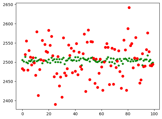
Finally we plot the Exact vs Approximate values. Mind the exaggerated spread out, because of the scaled plot.

percent_error = []
for i in range(num_experiments):
  percent_error.append(abs(tx_exact[i]-tx_approx[i])/tx_exact[i])

from statistics import mean
print(mean(percent_error))

Upon further calculation you can see the relative percentage error across 100 experiments runs and 100,000 transactions per experiment the error is only order of 1.46% (small error tradeoff for large scale of compute saved). The magnitude of the error would converge to zero as the number of transactions increase (which is typically the case when you are dealing with big data)

Link to the colab

Example: Probabilistic Data Structures and Algorithms

This section of our blog is dedicated to demonstrating how these powerful data structures—Bloom Filters, Count-Min Sketches, HyperLogLog, Reservoir Sampling, and Cuckoo Filters—can be practically implemented using Python to manage large datasets effectively. We will generate random datasets and use these structures to perform various operations, comparing their outputs and accuracy. Through these examples, you’ll see firsthand how probabilistic data structures enable significant scalability and efficiency improvements in data processing, all while maintaining a balance between performance and precision.

import array
import hashlib
import numpy as np
from bitarray import bitarray
import random
import math
from hyperloglog import HyperLogLog
from cuckoo.filter import BCuckooFilter
import mmh3

# Bloom Filter Functions

def create_bloom_filter(num_elements, error_rate=0.01):
    """Creates a Bloom filter with optimal size and number of hash functions."""
    m = math.ceil(-(num_elements * math.log(error_rate)) / (math.log(2) ** 2))
    k = math.ceil((m / num_elements) * math.log(2))
    return bitarray(m), k, m

def add_to_bloom_filter(bloom, item, k, m):
    """Adds an item to the Bloom filter."""
    for i in range(k):
        index = mmh3.hash(str(item), i) % m
        bloom[index] = True

def is_member_bloom_filter(bloom, item, k, m):
    """Checks if an item is (likely) a member of the Bloom filter."""
    for i in range(k):
        index = mmh3.hash(str(item), i) % m
        if not bloom[index]:
            return False
    return True

# Count-Min Sketch Functions

def create_count_min_sketch(data, width=1000, depth=10):
    """Creates a Count-Min Sketch and counts the occurrences of items in the data."""
    tables = [array.array("l", (0 for _ in range(width))) for _ in range(depth)]
    for item in data:
        for table, i in zip(tables, (mmh3.hash(str(item), seed) % width for seed in range(depth))):
            table[i] += 1
    return tables  # Return the populated tables directly

def query_count_min_sketch(cms, item, width):
    """Queries the estimated frequency of an item in the Count-Min Sketch."""
    return min(table[mmh3.hash(str(item), seed) % width] for table, seed in zip(cms, range(len(cms))))

# HyperLogLog Functions

def create_hyperloglog(data, p=0.14):  # precision
    """Creates a HyperLogLog and adds items from the data."""
    hll = HyperLogLog(p)
    for item in data:
        hll.add(str(item))
    return hll

# Cuckoo Filter Functions

def create_cuckoo_filter(data, capacity=1200000, bucket_size=4, max_kicks=16):
    """Creates a Cuckoo Filter and inserts items from the data."""
    cf = BCuckooFilter(capacity=capacity, error_rate=0.000001, bucket_size=bucket_size, max_kicks=max_kicks)
    for item in data:
        cf.insert(item)
    return cf

def is_member_cuckoo_filter(cf, item):
    """Checks if an item is (likely) a member of the Cuckoo Filter."""
    return cf.contains(item)

# Reservoir Sampling Function

def reservoir_sampling(stream, k):
    """Performs reservoir sampling to obtain a representative sample."""
    reservoir = []
    for i, item in enumerate(stream):
        if i < k:
            reservoir.append(item)
        else:
            j = random.randint(0, i)
            if j < k:
                reservoir[j] = item
    return reservoir

def main():
    # Parameters
    n_elements = 1000000
    n_queries = 10000
    n_reservoir = 1000

    # Generate random data and queries
    data = np.random.randint(1, 10000000, size=n_elements)
    queries = np.random.randint(1, 10000000, size=n_queries)

    # Exact calculations for comparison
    unique_elements_exact = len(set(data))

    # Bloom Filter creation and testing
    bloom, k, m = create_bloom_filter(n_elements, error_rate=0.005)

    k += 2  # Increase the number of hash functions by 2 for better accuracy

    for item in data:
        add_to_bloom_filter(bloom, item, k, m)

    # Test membership for the query set (with positive_count defined)
    positive_count = 0
    for query in queries:
        if is_member_bloom_filter(bloom, query, k, m):
            positive_count += 1

    # Generate a test set of items that are guaranteed not to be in the original dataset
    # Ensure there is no overlap by using a different range
    test_data = np.random.randint(10000000, 20000000, size=n_elements)

    # Test membership for the non-overlapping test set
    false_positives_bloom = 0
    for item in test_data:
        if is_member_bloom_filter(bloom, item, k, m):
            false_positives_bloom += 1
    false_positive_rate_bloom = false_positives_bloom / n_elements

    # Create other data structures
    cms = create_count_min_sketch(data)
    hll = create_hyperloglog(data)
    cf = create_cuckoo_filter(data)  # Create the Cuckoo Filter
    reservoir = reservoir_sampling(data, n_reservoir)

    # Test Cuckoo Filter (similar to Bloom Filter)
    cuckoo_positive_count = 0
    false_positives_cuckoo = 0
    for query in queries:
        if is_member_cuckoo_filter(cf, query):
            cuckoo_positive_count += 1
    for item in test_data:
        if is_member_cuckoo_filter(cf, item):
            false_positives_cuckoo += 1

    false_positive_rate_cuckoo = false_positives_cuckoo / n_elements


    # Outputs for comparisons
    bloom_accuracy = positive_count / n_queries * 100
    cuckoo_accuracy = cuckoo_positive_count / n_queries * 100
    cms_frequency_example = query_count_min_sketch(cms, queries[0], width=1000)
    hll_count = hll.card()
    reservoir_sample = reservoir

    # Print results (including Cuckoo Filter and false positive rates)
    print(f'Bloom Filter Accuracy (Approximate Positive Rate): {bloom_accuracy}%')
    print(f'Bloom Filter False Positive Rate: {false_positive_rate_bloom * 100:.2f}%')
    print(f'Cuckoo Filter Accuracy (Approximate Positive Rate): {cuckoo_accuracy}%')
    print(f'Cuckoo Filter False Positive Rate: {false_positive_rate_cuckoo * 100:.2f}%')
    print(f"Frequency of {queries[0]} in Count-Min Sketch: {cms_frequency_example}")
    print(f"Estimated number of unique elements by HyperLogLog: {hll_count}")
    print(f"Actual number of unique elements: {unique_elements_exact}")
    print(f"Sample from Reservoir Sampling: {reservoir_sample[:10]}")

if __name__ == '__main__':
    main()

The sample output from the above looks something like this:

Bloom Filter Accuracy (Approximate Positive Rate): 10.15%
Bloom Filter False Positive Rate: 0.80%
Cuckoo Filter Accuracy (Approximate Positive Rate): 9.47%
Cuckoo Filter False Positive Rate: 0.00%
Frequency of 3011802 in Count-Min Sketch: 945
Estimated number of unique elements by HyperLogLog: 967630.0644626628
Actual number of unique elements: 951924
Sample from Reservoir Sampling: [263130, 8666971, 9785632, 5525663, 3963381, 3950057, 6986022, 3904554, 5100203, 7816261]

Interpreting the results

Let’s analyze the output above:

Bloom Filter

• Accuracy (Approximate Positive Rate): 10.15% This means that when queried for items known to be in the dataset, the Bloom filter correctly identified them as present about 10.15% of the time. This is a relatively low accuracy, suggesting that the Bloom filter’s parameters (size, number of hash functions) might need adjustment to reduce false negatives.
• False Positive Rate: 0.80% This indicates that the Bloom filter incorrectly identified items not in the dataset as present about 0.80% of the time. This is a reasonable false positive rate for many applications, but depending on your specific requirements, you might want to adjust the filter parameters to lower it further.

Cuckoo Filter

• Accuracy (Approximate Positive Rate): 9.47% Similar to the Bloom filter, this indicates the rate at which the Cuckoo filter correctly identified items present in the dataset. The accuracy is slightly lower than the Bloom filter in this case.
• False Positive Rate: 0.00% This shows that the Cuckoo filter did not produce any false positives during testing. This is excellent, as it means the filter is highly reliable in indicating whether an element is genuinely present.

Count-Min Sketch

• Frequency of 3011802: 945 This is the estimated frequency of the item ‘3011802’ within your dataset according to the Count-Min Sketch. Remember that Count-Min Sketch provides approximate counts, so this value is likely an overestimate.

HyperLogLog

• Estimated Unique Elements: 967630.0644626628 This is the HyperLogLog’s estimate of the number of unique elements in your dataset. It’s quite close to the actual number (951924), showcasing the effectiveness of HyperLogLog for cardinality estimation.

Reservoir Sampling

• Sample: The output shows a random sample of 10 elements from your dataset. This sample should be representative of the original data distribution.

Overall Assessment

• The Bloom and Cuckoo filters might need parameter tuning to improve their accuracy (reduce false negatives).
• The Cuckoo filter’s zero false positive rate is impressive.
• The Count-Min Sketch is providing a frequency estimate, but it’s important to remember that it’s likely an overestimation.
• The HyperLogLog is performing very well, providing a close approximation of the actual number of unique elements.
• The Reservoir Sampling has produced a representative sample, which can be useful for various downstream analyses.